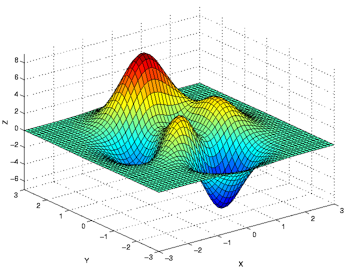
Plot of the Matlab peaks() function; a sample function for 3d graphics built from translated and scaled Gaussians.
Plot of the Matlab peaks() function; a sample function for 3d graphics built from translated and scaled Gaussians.
In general, Matlab is run by selecting the application from a menu, or typing matlab at the command line prompt in a UNIX environment. Once running, Matlab is itself a command line program, wherein you will be given a prompt to type in specific commands.
You should see a graphics window flash up on the screen and then disappear. If so, you are all set; otherwise you need to check that you have set your display variables properly. If you can't get the graphics to appear on the screen, Matlab should work, but without any plotting.
To see the graphics window, you just need to plot something. Try typing
>> plot(1:0.5:5)
which will plot the numbers 1 to 5 (counting by 0.5) by their index (1 to 9). As you'll see later, the colon (:) is a shorthand for creating a vector of numbers. You will use it a lot in Matlab.
Matlab is a program for doing scientific calculations using matrices. The matrix is the basic data type of matlab, and it may be real or complex. Matlab only uses double-precision floating point numbers; there are no integer matrices. You can also use scalars (1 x 1 matrices) or vectors (n x 1 or 1 x n matrices). What makes Matlab very powerful is that you can perform operations on whole vectors or matrices at one time, without having to loop through each element. Matlab is also quite good at plotting data (in 2- and 3-d), which makes it useful for plotting data generated elsewhere.
In this tutorial, we'll go over some of the basic commands, how to read in data, how to save data, how to plot data, and how to create simple programs, called m-files.
If you get stuck or just need more information about Matlab, there are a number of different resources. The easiest one to use is built into Matlab itself. By typing help or help command, you can get a description of a command or group of commands. Try typing
>> help graph2d
This gives you a list of all of the 2-dimensional plotting functions available. Another helpful command is the lookfor command. By typing lookfor keyword, you will get a list of all commands related to keyword, even if you aren't sure of the exact function name.
There are also a number of books, including the Matlab manual and Getting Started in Matlab by Rudra Pratap.
The Mathworks (developers of Matlab) WWW site, http://www.mathworks.com, has extensive documentation available (under Support). The documentation for Matlab (but not the toolboxes or other Mathworks products) is available here. For users who wish to kill a forest of trees for paper manuals, they are available for order from Mathworks, or as PDF files on the web here.
Here's a short tutorial on working with variables, taken from the book, Getting Started in Matlab. It is highly recommended that you obtain this book as it will make your life in Matlab easier. Variables in Matlab can have any name, but if the variable has the same name as a function, that function will be unavailable while the variable exists. Try typing the following into Matlab:
>> 2+2					% Add two numbers
					%
ans =					% Matlab uses 'ans' if
					% there is no variable
     4					% assignment (lvalue)

>> x= 2+2				% Assigns the result
					% to variable 'x'
x =					% and displays the
					% value of 'x'
     4					%

>> y=2^2 + log(pi)*sin(x);		% The semicolon at
>> y					% the end suppresses output
					% To see the value of a
y =					% variable, enter just its'
					% name
    3.1337

>> theta=acos(-1)			% Assign arccos(-1) to theta
					% Matlab uses radian for all
theta =					% trig functions

    3.1416

>> theta-pi				% Note that pi is built into
					% Matlab, and more precision
ans =					% is kept internally than is
					% printed on the screen
     0
In Matlab, there are a number of ways to create matrices. First, let's look at how to generate vectors (call them x and y), which are 1xN matrices. We will make x go from 0 to 3*pi.
>> x=0:0.1:3*pi;		% Create vector x from 0 to 3*pi in
				% increments of 0.1
				% But, could also use:
>> x = linspace(0,3*pi,100);	% Create vector x from 0 to 3*pi with
				% 100 steps exactly
>> beta=0.5;			% Create constant beta for error function
>> y=beta*erf(x/5);		% Compute erf() for each x value, and
				% assign to a y value
				% Note that there is no loop here, but
				% y now has as many entries as x!
>> plot(x,y)			% Plot x vs. y with a line
The plot should look something like this.
Now, let's try making true two-dimensional matrices (MxN); start with a 3x3 matrix typed on the command line:
>> x = [1 4 7; 2 5 8; 3 6 9];		% semicolons denote changes of
					% row

>> x = [1,4,7				% Matlab's command line knows
2,5,8					% the matrix is not finished
3,6,9];					% until the closing ']'
In any case, the result is the same, the following 3 x 3 matrix stored as the variable x:
>> x				% Display the current value of x

x =

     1     4     7
     2     5     8
     3     6     9
You should notice that square brackets ([ ]) enclose the matrix, spaces or commas (,) denote elements within a row, and either a semicolon (;) or a hard return denote rows.
Matlab also has functions to produce matrices of zeros and ones of a specified size:
>> zeros([3 3])		% Produce matrix of all zeros,
			% size of 3x3
ans =

     0     0     0
     0     0     0
     0     0     0

>> zeros(3, 3)		% Alternate size format of above

ans =

     0     0     0
     0     0     0
     0     0     0

>> zeros(2)		% Matrix of zeros, size 2x2

ans =

     0     0
     0     0

>> zeros([1 2])		% Row vector of zeros, 2 long

ans =

     0     0

>> zeros([2 1])		% Column vector of zeros, 2 long

ans =

     0
     0

>> ones(2, 2)		% Same as zeros(), but matrix filled with 1

ans =

     1     1
     1     1
To access matrix elements, specify the rows and columns we are interested in. Remember how we used the colon (:) to fill in numbers when we plotted numbers from 1 to 5 in the first section? We will use that again. The syntax is x(row,col) so, for example, if we want the to assign the element in the third row, first column to the variable y, we type:
>> y = x(3,1); % Assign row 3, col 1 element of x to y
To specify an entire row or column, use a colon (:) in place of the row or column number. So, if we want the entire second column, we would type:
>> y = x(:,2); % Assign all rows, col 2 elements to y
Now let's try a short exercise to use matrices and matrix operations.
Here is a transcript (diary) of a matlab session implementing the exercise:
>> a=1:5;			% vector of 1 to 5, increment 1
>> a=a+1			% add 1 to all elements of a

a =

     2     3     4     5     6

>> b=5:-1:1			% vector of 5 to 1, increment -1

b =

     5     4     3     2     1

>> c=a+b			% add a and b, store in c

c =

     7     7     7     7     7
Note that all vectors used so far have been row vectors; the vector is a row from a matrix (one row, many columns). There are also column vectors, which are displayed vertically (many rows, one column). To transform a row vector to a column vector (or back), use the transpose operation; in Matlab, this is denoted by ' after the vector (or matrix) name.
>> a'

ans =

     2
     3
     4
     5
     6
Matlab, being focused on matrix operations, always assumes operations are matrix operations unless told otherwise. In the exercise above, we added a scalar to a matrix, which is the same as adding a scalar to every element of the matrix. In general, though, Matlab will do matrix addition, multiplication, division, etc.
To make Matlab apply an operation to each element individually (rather than use matrix operations), use a .(period) before the operator; for example, to square each element of a vector, we use:
>> a=1:5;
>> a.*a				% the . makes Matlab apply the *
				% to each element as a set of scalar
ans =				% operations, NOT matrix multiplication

     1     4     9    16    25
If there is no ., Matlab assumes the intent is a matrix operation, which won't work for two row vectors:
>> a*a
??? Error using ==> *
Inner matrix dimensions must agree.
If the intent really is to do a matrix multiplication of a by a, we need to take the transpose of the second vector:
>> a*a'

ans =

    55
Since a is a 1x5 vector, a' (transpose of a) is a 5x1 vector. When multiplied, the result is a 1x1 vector, which is a scalar, as seen here.
Keeping track of matrix dimensions can be difficult, but is extremely important. Fortunately, Matlab will normally produce errors when your code tries to do something mathematically incorrect.
Matlab has a very general indexing ability, which can make code that is compact and efficient, but less transparent. In general, anywhere you can index a matrix with a single number (or set of numbers), you can also index with a vector or matrix. Some examples:
EDU>> a=[1:3; 4:6; 7:9]         % Create 3x3 matrix

a =

     1     2     3
     4     5     6
     7     8     9

EDU>> a(:)                      % Access matrix as a vector.
                                % Note that the elements are taken
ans =                           % from each column first, then each
                                % row.  This format allows the treatment
     1                          % of any multi-dimensional array as a
     4                          % vector, which can be useful for some
     7                          % function calls.
     2                          % 3+ dimensional arrays will take elements
     5                          % first from the last dimension, working
     8                          % back to the first dimension!
     3
     6
     9

EDU>> b=[1:10].^2

b =

     1     4     9    16    25    36    49    64    81   100

EDU>> b(a)                      % Access elements of b using values of a.
                                % Note that the result is a matrix with the
ans =                           % same shape as a, but with values taken from
                                % b; the entries of a are used as indexes
     1     4     9              % into the vector b.  Matlab will produce an
    16    25    36              % error if any index from a is outside the
    49    64    81              % bounds of b.

EDU>> a                         % Reminder of entries of matrix a

a =

     1     2     3
     4     5     6
     7     8     9

EDU>> b=flipud(a)

b =

     7     8     9
     4     5     6
     1     2     3

EDU>> b(a)                      % Access elements of b using values of a.
                                % Note that the elements were taken in
ans =                           % column-order (elements 1-3 are the first
                                % column).  This comes from Matlab treating
     7     4     1              % b as a vector for the indexing operation,
     8     5     2              % with the resulting vector reshaped to the
     9     6     3              % size of a.
These examples are all designed to show how Matlab stores and retrieves
information in arrays. Matlab stores all arrays as a long vector in
memory, regardless of the number of dimensions. A multi-dimensional
array (a matrix) is stored as a vector, with additional information on
how many rows and columns are in the matrix, so Matlab can quickly
access any element using (row, column) indexing. The translation for a
2-D matrix (nr x nc elements) is simple:
A(i,j) == A(j*nr + i)where nr is the number of rows in the matrix. A 3-D array (n1 x n2 x n3 elements) is similar:
A(i,j,k) == A((k*n1*n2) + (j*n2) + i)where n1 is the stride for the last dimension, and n2 is the stride for the second dimension.
Given this memory layout for a multi-dimensional matrix, it is clear why accessing the matrix as a vector (using the A(:) notation) results in a vector with columns attached end-to-end; Matlab is starting at the first element and reading straight through until the end. This sort of indexing, once understood, can make some very efficient algorithms. For example, translating gray scale values in an image from one scale to another:
EDU>> A = floor(rand(10)*255)   % Create random 10x10 matrix
                                % of 8-bit gray scale values
A =                             % [0-255].

     3    67   137   173    18   211   192   118    46     6
    73   192   158    18    49   233   169   233   127   221
   208   168   174    18    96    28   225    58   107     6
   251    54   172     3    70   207    69   219   168   132
     4   153   223    57   196   231   106   167   171    49
   208   154     3   131    80    39    54   227   244   182
   158   168    79   116   162    31     9   124    48    63
   142    46   198   179   251   194    20   253    28   238
    62   162    78   148   128   184   216    95   144    34
   209    43   236   129   241   166    86   135   247   133

EDU>> B = [0:2:100 linspace(101,199,256-80) 200:2:256]; size(B)
                                % Create new gray scale mapping
ans =                           % that compresses the ends and
                                % expands the middle of the
     1   256                    % spectrum; must be 256 entries!

EDU>> floor(B(A+1))             % Remap A by choosing entries of
                                % the new map (B) accoding to values
ans =                           % in A. Note the addition of 1, to
                                % shift [0-255] to [1-256].
     4   109   148   168    34   190   179   137    90    10
   112   179   160    34    96   210   166   210   143   195
   188   165   169    34   125    54   197   104   131    10
   246   102   168     4   111   187   110   194   165   145
     6   157   196   103   181   206   131   165   167    96
   188   158     4   145   116    76   102   199   232   173
   160   165   116   136   162    60    16   141    94   107
   151    90   182   172   246   180    38   250    54   220
   106   162   115   154   143   174   192   125   152    66
   188    84   216   144   226   164   120   147   238   146
This efficient, but less transparent, implementation of a remapping
could also be done via for loops (one or two, depending on
implementation), but that would be much, much slower for large
matrices.
The key to loading data into Matlab is to remember that Matlab only uses matrices. That means that if you want to easily read a data set into Matlab, all of the rows must have the same number of elements, and they must all be numbers.
Most commonly, you'll be dealing with a text (ASCII) file. If you have a set of data on disk in a file called points.dat, then to load it, you would type:
>> load points.dat
This will load your data into the Matlab variable points. Let's assume that the file points.dat contains two columns, where column 1 is height and column 2 is distance. To break apart points into something more meaningful, we use:
>> height = points(:,1);
>> distance = points(:,2);
This creates a vector height from the first column (all rows), and distance from the second column.
To save the same data into an ASCII file called mydata.dat, we use either:
>> save mydata.dat height distance -ascii	% common form for
						% command line
or
>> save('mydata.dat', 'height', 'distance', '-ascii');
						% common form for
						% use in scripts and
						% functions
The -ascii flag is important here; it tells Matlab to make the file in ASCII text, not a platform-independant binary file. Without the flag, the file would be unreadable with standard editors. Text is the most portable and editable format, but is larger on disk. Matlab's binary format is compatible across all platforms of Matlab (Windows, UNIX, Mac, etc.), and is more compact than text, but cannot be edited outside of Matlab.
You will note that when Matlab saves files in ASCII format, it uses scientific notation whether it needs it or not.
More powerful and flexible save and load schemes exist in Matlab; they use the fprintf() and fscanf() functions along with fopen() to control file output. A discussion of the intricacies of using fscanf/fprintf is beyond this tutorial; see the help pages or someone with firsthand experience.
Now that we can save, load, and create data, we need a way to plot it. The main function for making 2-dimensional plots is called plot. To create a plot of two vectors x and y, type plot(x,y). With only one argument (plot(x)) plot will plot the argument x as a function of its index. If x is a matrix, plot will produce a plot of the columns of x each in a different color or linestyle. More detail on the basic use of plot is available via the help plot command in Matlab.
That brings us to the third possible argument for plot, the linestyle. plot(x,y,s) will plot y as a function of x using linestyle s, where s is a 1 to 3 character string (enclosed by single quotes) made up of the following characters.
y yellow	.  point
m magenta	o  circle
c cyan		x  x-mark
r red		+  plus
g green		-  solid
b blue		*  star
w white		:  dotted
k black		-. dashdot
		-- dashed
For example, to create a plot of x versus y, using magenta circles, type the command plot(x,y,'mo');. To plot more than one line, you can combine plots by typing plot(x1,y1,s1,x2,y2,s2,...);.
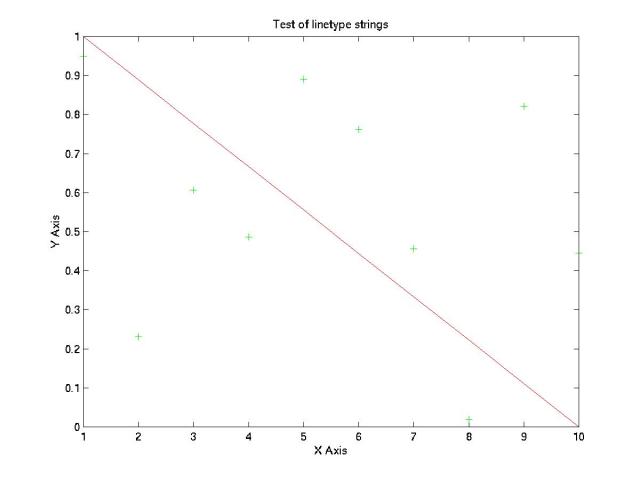
As an example, plot a random vector (10 x 1) and an integer vector from 1 to 10 using two different line types:
>> y1=rand(10,1);
>> y2 = linspace(1,0,10);
>> x = 1:10;
>> plot(x, y1, 'g+', x, y2, 'r-');
>> title('Test of linetype strings');
>> xlabel('X Axis');
>> ylabel('Y Axis');
The plot should look something like this:
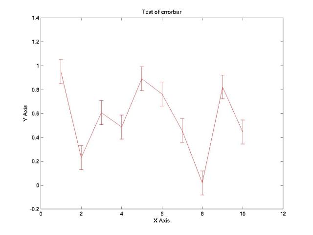
Another useful plotting command is called errorbar. The following example will generate a plot of the random vector y1 using an error of 0.1 above and below the line:
>> errorbar(x,y1,ones(size(y1)).*0.1,'r-')
>> title('Test of errorbar');
>> xlabel('X Axis'); ylabel('Y Axis');
The plot should now look something like this:
title, xlabel, and ylabel create labels for the top and sides of the plot. They each take a string variable, which must be in single quotes. One other labelling function that might be useful is the text function. The command text(1,10,'Here is some text'); will write the text string 'Here is some text' at the (x,y) position (1,10) in data units.
One thing you might want to do with your plot is to change the axes. Normally, Matlab automatically chooses appropriate axes for you, but they're easy to change. The axis command will allow you to find out the current axes and change them.
>> axis						% Get the current axis
						% settings
ans =

         0   12.0000   -0.2000    1.4000

>> axis([2 10 -0.2 1.0])			% Reset axes extents to
						% [xmin xmax ymin ymax]
Sometimes you will want to switch the position of the plot origin (normally used for plotting images of matrices). Typing
>> axis('ij')
will switch the Y axis direction so that (0,0) is to the upper right.
Sometimes it's useful to be able to add something to a plot window without having to draw two lines with the same plot statement (as we did above). So Matlab has a command, hold which will cause the plot to remain (it doesn't redraw it). Typing hold on will hold the current plot, and hold off will release the plot. Also, hold by itself will toggle the hold state. You might also want to use clf to clear the graphics window and release the window.
For those of you that will use Matlab to make plots for publications and presentations will greatly benefit from a few useful but poorly documented Matlab functions. The commands get and set allow the user to check or tweak a plot into more pleasing form. For example by using these commands, one can change font sizes, colors, line widths and axes labels as well as many other plot attributes.
We will start by generating a simple plot:
>> x = [0:100]*pi/50;
>> y = sin(x);
All the attributes of a plot are stored in a data structure which may be obtained by typing:
>> p = plot(x,y)
By giving a plot an output varible, you have obtained the object handles. In order to find out what handles exist we use the get command.
>> get(p)
A list will be printed out which is partially listed below:
	Color = [0 0 1]
	EraseMode = normal
	LineStyle = -
	LineWidth = [0.5]
	...
If you wish to obtain the value to just one axis handle, for example the line style, this can be done by typing:
>> get(p,'LineStyle')
ans =
-
Each of these is a graphic handles that may be changed by using the command set. For example, suppose that we now wish to make the plot red instead of blue and increase the line width from 0.5 to 1.
>> set(p,'Color',[1 0 0],'LineWidth',1);
Any graphic handle may be changed using this method. As you begin to use Matlab, these commands may not be used often, but as you become more proficient, you may find these commands to be invaluable. Other attributes of a plot can be changed by using gca (for axes properties) and gcf (for figure window properties). Type get(gca) and get(gcf) to see what other attributes may be changed. And like any other part of Matlab, these commands may be added to scripts to created custom plots.
In Matlab, you can create a file using Matlab commands, called an m-file. The file needs to have a .m extension (hence the name -- m-file). There are two types of m-files: (1) scripts and (2) functions. We will start with scripts, as they are easier to write.
Running a Matlab script is the same as typing the commands in the workspace. Any variables created or changed in the script are changed in the workspace. A script file is executed by typing the name of the script (without the .m extension). Script files do not take or return any arguments, they only operate on the variables in the workspace. If you need to be able to specify an argument, then you need to use a function. Here is an example of a simple script to plot a function:
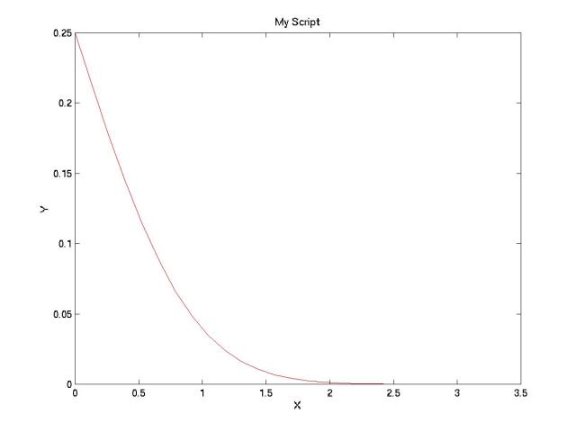
% makefunction.m
% script to plot erfc in domain [0,pi]

x = linspace(0,pi,25);		% Create x from 0 to pi with 25 values
y = erfc(x);			% Calc. erfc of x
scl = 0.25;			% Plotting scaling factor
y = y*scl;
plot(x,y, 'r-');		% Plot x and y
title('My Script');		% Create a title
xlabel('X');			% Label the x and y axes
ylabel('Y');
Note the use of '%' characters to introduce comments, just as in the examples throughout this tutorial. In general, Matlab treats anything after a '%' as if it wasn't there; comments are silently ignored. This can be very useful when writing m-files, as debugging commands can be commented out after the m-file is tested.
Running this m-file produces the following variables in the workspace and plot (in a separate window):
>> whos				% Empty workspace; no variables defined
>> makefunction			% Create vars, plot
>> whos				% List vars in workspace
  Name      Size         Bytes  Class

  scl       1x1              8  double array
  x         1x25           200  double array
  y         1x25           200  double array

Grand total is 51 elements using 408 bytes
You should notice that all of the variables used in the script are now sitting in the workspace, so that they can be used again. This is exactly the same as if they had been typed in separately. Anytime a computation is going to take more than a single line, it is worthwhile to create a throwaway m-file; the file can be saved, edited, and revised much easier than using just the command line.
Matlab functions are very similar to scripts, but they can accept and return values as arguments. Most of the commands available in Matlab are actually pre-written Matlab functions; only a small number of important functions are compiled into the program (e.g. matrix multiply).
To write a function, create an m-file with a function declaration as the first line (see the example, below). The return values in the declaration will need to be set somewhere in the function body; whatever value these variables have at the end of the function will be returned.
Comments immediately after the function declaration will be used as the help page for the function; it should have useful information on function arguments and return values. If the function uses a special (named) algorithm, that is useful to put in the help as well.
Functions keep variables local; variables defined in the function are not part of the workspace, and the function cannot access variables in the workspace unless they are passed as arguments. Hence, functions can define a variable without worrying if it already exists. All variables in a function are lost once the function completes.
An example function definition (from a file named llsqErr.m):
function [mean, sigma] = llsqErr(x, y, N, dx, dy);
% function [mean, sigma] = llsqErr(x, y, N, dx, dy);
%
% Generate mean and s.d. of slope  and intercept
% for linear least-squares fit to x, y data set, using MC
% technique with random errors of scale dx, dy.  Random errors
% are uniformly distributed, and symmetric (with scale dx, dy)
% about x and y values.
%
% x, y are vectors of data, of length > 2
% dx, dy are scalars
% N is scalar (# of trials); typically should be >1e3
%
% Uses N trials with random perturbations computed for each trial
%
% Returns values as [slope intercept] for means and s.d.s

%% Notes %%
% This code really ought to guarantee that the randomly generated
% pertrubations are unique.  This is assumed from the use of a
% pseudo-random number generator, and the likely event that N is
% less than the recurrence interval of the PRNG.
%
% It appears necessary to compute the predicted errors for each
% data set individually; attempts to generate a general correlation
% plot didn't pan out.

m = zeros(N, 2);
for i=1:N
  xh = x + dx*(2*rand(size(x))-1); % generate perturbed x, y vecs
  yh = y + dy*(2*rand(size(y))-1);

  p = polyfit(xh, yh, 1); % get slope, intercept
  m(i, :) = p; % store
  end

mean  = [ mean(m(:,1)) mean(m(:,2)) ];
sigma = [ std(m(:,1))  std(m(:,2)) ];
This function accepts 5 arguments: x, y, N, dx, and dy. It returns two vectors: mean and sigma. Note that the comments after the function declaration indicate what the arguments and return values are, as well as how the function does its' work. Also note that there are comments about possible problems with this algorithm and implementation. A user looking at the source code for this function can determine what is happening, and what might need to be changed. Also note that the function uses simple variable names, which could exist in the workspace (x, y, etc.); because this is a function, the variables used are not part of the workspace, so there are no concerns.
When a user gets help for this function, the first set of comments (up to the blank line) is returned as the help page:
>> help llsqErr

  function [mean, sigma] = llsqErr(x, y, N, dx, dy);

  Generate mean and s.d. of slope  and intercept
  for linear least-squares fit to x, y data set, using MC
  technique with random errors of scale dx, dy.  Random errors
  are uniformly distributed, and symmetric (with scale dx, dy)
  about x and y values.

  x, y are vectors of data, of length > 2
  dx, dy are scalars
  N is scalar (# of trials); typically should be >1e3

  Uses N trials with random perturbations computed for each trial

  Returns values as [slope intercept] for means and s.d.s
One other useful command is the diary command. Typing
>> diary filename.txt
will create a file with all the commands you've typed. When you're done, typing
>> diary off
will close the file. This might be useful to create a record of your work to hand in with a lab or to create the beginnings of an m-file.
At this point, you should know enough to maneuver around in Matlab and find whatever else you need. Help is available from the built-in help command, the on-line help system at www.mathworks.com, or fellow students and faculty.